Key points
- Decay is random and spontaneous: the half-life is fixed, but the timing of any one decay is not.
- Activity A = λN, measured in becquerels (decays per second).
- N = N₀e^(−λt) and A = A₀e^(−λt) have the same shape, with λt½ = ln 2.
- A graph of ln A against t is a straight line with gradient −λ.
- Subtract background before using count rates in half-life calculations.
What radioactive decay is
Radioactive decay is the process by which an unstable nucleus emits radiation and changes into a different nucleus. If you want the radioactive decay equation and half-life in one idea, it is this: every nucleus has the same fixed chance of decaying in each second, so the number of undecayed nuclei falls exponentially.
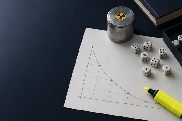
Two words matter in the OCR A specification. Decay is random, which means you cannot predict when one particular nucleus will go. It is also spontaneous, which means it is not triggered by anything outside the nucleus. Heating the sample, compressing it or putting it in a chemical reaction does not change how quickly it decays.
Randomness sounds like it should make the maths messy, but the opposite is true. With billions of nuclei, the random behaviour averages out into a smooth, predictable curve. That is why we can talk about a half-life even though no single nucleus has a schedule.
The rest of this guide builds the idea in the order you will meet it in exam questions: activity and the decay constant, the exponential equations, half-life, the graphs (including ln graphs), how you measure decay in a lab, how to model it with dice or a spreadsheet, and carbon dating. Everything links back to the same one-line idea about a constant chance of decay.
Activity and the decay constant
The activity A of a source is the number of nuclei that decay per second. Its unit is the becquerel (Bq), where 1 Bq is one decay per second. Do not confuse activity with the count rate on a detector. The detector only catches a fraction of the radiation, so the count rate is lower than the true activity.
The decay constant λ is the probability that an individual nucleus decays per unit time. A large λ means the nuclei are very unstable and the source dies away quickly. A small λ means a long-lived source. Its unit is s⁻¹ (or h⁻¹, y⁻¹ if time is measured in hours or years).
If each nucleus has chance λ of decaying per second and there are N nuclei, the number decaying per second is λN. The minus sign in dN/dt appears because N is falling.
A = −dN/dt = λN
- A = activity / Bq
- λ = decay constant / s⁻¹
- N = number of undecayed nuclei present
A is proportional to N. When N halves, A halves.
This proportionality is the key to everything else. Activity is proportional to the number of undecayed nuclei, so the activity falls in exactly the same exponential pattern as N does. The same is true of the count rate on a detector, as long as the detector and source stay in the same positions.
Half-life and the exponential equations
The half-life t½ is the average time taken for half of the undecayed nuclei in a sample to decay. Equivalently, it is the time for the activity to fall to half its initial value. It is constant for a given isotope: after one half-life you have 1/2, after two you have 1/4, after three you have 1/8.
Because the rate of decay is proportional to N, the solution is an exponential. You are expected to use these in the form given in the data and formulae booklet.
N = N₀e^(−λt)
- N₀ = number of undecayed nuclei at t = 0
- N = number at time t
- λ = decay constant / s⁻¹
- t = time / s
A = A₀e^(−λt)
The same law holds for activity, and for the corrected count rate C = C₀e^(−λt).
To link λ and half-life, put N = N₀/2 when t = t½. Then N₀/2 = N₀e^(−λt½), so ½ = e^(−λt½). Take natural logs of both sides: ln(½) = −λt½, and since ln(½) = −ln 2, you get:
λt½ = ln 2 (so t½ = 0.693 / λ)
Check the units match: if t½ is in hours, λ must be in h⁻¹.
You should be able to give this short derivation, not just quote it. Notice that it never mentions N₀, which is why half-life does not depend on how much sample you start with.
Decay graphs and ln graphs
A graph of N (or A, or count rate) against time is a decaying exponential. It starts at N₀ and never quite reaches zero. The gradient at any point is −λN, so the curve gets shallower as N falls. You can read a half-life straight off it: find the time for the value to fall from any point to half of that value. Check at least two different starting points. If the half-life is the same each time, the curve is exponential.
A curve is hard to measure accurately, so examiners like the straight-line version. Take natural logs of A = A₀e^(−λt):
ln A = ln A₀ − λt
Compare with y = mx + c: plot ln A on the y-axis and t on the x-axis.
A graph of ln A against t is a straight line with gradient −λ and intercept ln A₀. The gradient is negative, so λ is the magnitude of the gradient. Then you can find t½ from λt½ = ln 2.
Two details cost marks. First, ln has no unit, so the axis label is ln (A / Bq), not ln A (Bq). Second, if the data has background subtracted, say so. Taking logs of uncorrected counts gives a line that bends towards the background level at long times. Use a large triangle for the gradient, using points on the line, not data points that sit off it.
Randomness, background and measuring decay
Evidence that decay is random comes from a detector such as a Geiger-Müller tube. Place it near a source and the counts arrive at irregular intervals, and the number in repeated equal time intervals fluctuates around an average. Evidence that decay is spontaneous is that the rate does not change when you change the temperature or pressure of the source.
Background radiation comes from rocks, air (radon), cosmic rays, buildings and medical sources. It is always present, so you must measure it with the source removed and subtract it. Measure the background over a long time, say several minutes, and take an average, because it is also random and a short measurement is unreliable.
- Measure the background count rate with no source nearby.
- Measure the count rate with the source at a fixed distance.
- Subtract the background rate to get the corrected count rate.
- Repeat at intervals and plot corrected count rate against time, or ln(corrected count rate) against time.
Because decay is random, the count itself has scatter. A larger number of counts gives a smaller percentage uncertainty, so count for longer when the source is weak. For a half-life of seconds, such as a short-lived gas produced in a bottle, the readings must be taken quickly, so repeat the experiment and average the results.
Modelling decay with dice and iteration
A classroom dice model shows how a constant chance gives an exponential. Start with a large number of dice, each one a 'nucleus'. Throw them all. Remove every die that shows a six, as these have 'decayed'. Count the survivors, then throw the survivors again. Each throw is one time step. The chance of decay per step is 1/6, so on average the number left falls by a factor of 5/6 each throw.
Plot survivors against throws and you get a noisy exponential. With only 30 dice the scatter is large. With a hundred or more, the curve is much closer to the smooth one. The model also lets you find a 'half-life' in throws: the time for the survivors to halve, which is about 3.8 throws here, since (5/6)ⁿ = 0.5 gives n = ln 0.5 / ln(5/6) = 3.8.
A spreadsheet or iterative model does the same job without dice. In a small time step Δt, the number of nuclei that decay is approximately λNΔt, so:
ΔN = −λNΔt
- ΔN = change in N during the time step
- Δt = time step, which must be small compared with the half-life
Use N(new) = N(old) + ΔN, and repeat. This is a numerical method for solving the exponential law.
The iteration slightly underestimates N because it assumes the activity stays at its start-of-step value for the whole step, when in reality it is falling. Halving the step makes the answer closer to the exact one. You are unlikely to be asked to write code, but you may be asked to complete a table of values or to comment on the effect of changing Δt.
Carbon dating and the three radiations
Living organisms take in carbon from the atmosphere, including a small, nearly constant fraction of radioactive carbon-14. While alive, the proportion stays steady because new carbon-14 replaces what decays. When the organism dies, intake stops, and the carbon-14 decays with a half-life of about 5730 years (use the value given in the question). Compare the activity per gram of carbon in an old sample with that of living material, and you can estimate the age with A = A₀e^(−λt), rearranged to t = (1/λ) ln(A₀/A).
The method has limits. It only works for once-living material, works best over a few half-lives (a very old sample has too little carbon-14 left to count reliably) and assumes the atmospheric proportion was the same in the past. Low activity also means a large percentage uncertainty from random counting.
| Alpha (α) | Beta-minus (β⁻) | Gamma (γ) | |
|---|---|---|---|
| What it is | Helium nucleus: 2 protons, 2 neutrons | Fast electron from a neutron changing to a proton | Photon from an excited nucleus |
| Charge | +2e | −e | 0 |
| Range in air | A few centimetres | About a metre | Long; falls off with distance |
| Stopped by | Paper, skin | A few mm of aluminium | Thick lead or concrete reduces it |
| Ionising power | Strongest | Medium | Weakest |
| Deflected by a magnetic field | Yes, slightly | Yes, strongly | No |
In an alpha decay the nucleus loses 4 nucleons and 2 protons, so the nucleon number falls by 4 and the proton number by 2. In beta-minus decay a neutron becomes a proton, so the nucleon number is unchanged and the proton number rises by 1, and an antineutrino is also emitted. Gamma emission changes neither number. For energy balance and conservation rules in nuclear equations, see binding energy and mass defect. The deflection of beta particles and alpha particles in a field uses the ideas in magnetic fields and flux density.
Worked examples
Activity from the number of nuclei
A radioactive sample has a half-life of 6.0 hours and contains 3.0 × 10¹⁵ undecayed nuclei. Calculate its activity.
- Convert the half-life to seconds: t½ = 6.0 × 3600 = 2.16 × 10⁴ s.
- Use λt½ = ln 2: λ = 0.693 / 2.16 × 10⁴ = 3.21 × 10⁻⁵ s⁻¹.
- Use A = λN: A = 3.21 × 10⁻⁵ × 3.0 × 10¹⁵ = 9.63 × 10¹⁰ Bq.
Answer A = 9.6 × 10¹⁰ Bq
Fraction left and time to reach 5%
An isotope has a half-life of 8.0 days. (a) What fraction of the nuclei remain after 20 days? (b) After how many days has the activity fallen to 5.0% of its initial value?
- λ = ln 2 / 8.0 = 0.0866 day⁻¹.
- (a) N/N₀ = e^(−λt) = e^(−0.0866 × 20) = e^(−1.733) = 0.177. Check: 20 days is 2.5 half-lives, and 0.5^2.5 = 0.177.
- (b) A/A₀ = 0.050 = e^(−λt), so −λt = ln 0.050 = −2.996.
- t = 2.996 / 0.0866 = 34.6 days.
Answer (a) 0.18 (b) 35 days
Carbon dating
Living wood gives a corrected count rate of 15.3 counts per minute for each gram of carbon. A sample of ancient wood gives 3.9 counts per minute per gram, after background correction. The half-life of carbon-14 is 5730 years. Calculate the age of the sample.
- λ = ln 2 / 5730 = 1.21 × 10⁻⁴ year⁻¹.
- A = A₀e^(−λt), so ln(A₀/A) = λt.
- ln(15.3 / 3.9) = ln 3.923 = 1.367.
- t = 1.367 / 1.21 × 10⁻⁴ = 1.13 × 10⁴ years.
Answer About 1.1 × 10⁴ years. Sense check: the activity fell by a factor of about 4, so about two half-lives, and 2 × 5730 is about 11 500 years.
Half-life from a ln graph
A student plots ln (A / Bq) against t / h for a source. The line passes through (0, 5.80) and (12, 3.40). Find (a) the decay constant, (b) the half-life and (c) the initial activity.
- (a) Gradient = (3.40 − 5.80) / 12 = −0.200 h⁻¹, so λ = 0.200 h⁻¹.
- (b) t½ = ln 2 / λ = 0.693 / 0.200 = 3.47 h.
- (c) ln A₀ = 5.80, so A₀ = e^5.80 = 330 Bq.
Answer (a) 0.20 h⁻¹ (b) 3.5 h (c) 3.3 × 10² Bq
Background correction
A GM tube gives a count rate of 540 counts per minute with a source in place. With the source removed the rate is 36 counts per minute. The source has a half-life of 10 minutes. What count rate would you expect to measure 30 minutes later?
- Corrected rate now = 540 − 36 = 504 counts per minute.
- 30 minutes is 3 half-lives, so the corrected rate becomes 504 / 8 = 63 counts per minute.
- The detector still picks up background, so the measured rate is 63 + 36 = 99 counts per minute.
Answer 99 counts per minute (the source contributes 63 of these)
Iterative model
A model for a sample uses ΔN = −λNΔt with N₀ = 1000, λ = 0.10 s⁻¹ and Δt = 1.0 s. Find N after three steps and compare it with the exact value at t = 3.0 s.
- Each step: ΔN = −0.10 × N × 1.0, so N is multiplied by 0.90.
- After step 1: N = 900. After step 2: N = 810. After step 3: N = 729.
- Exact: N = 1000e^(−0.10 × 3.0) = 1000e^(−0.30) = 741 (3 s.f.).
- The model is 12 lower, about 1.6% below the exact value, because it uses the activity at the start of each step.
Answer N = 729 from the model, 741 exactly. A smaller time step would reduce the difference.
Common mistakes
- Mixing units. Using t½ in hours with λ in s⁻¹. Convert one to match the other before you substitute.
- Forgetting background. Using raw counts in a half-life calculation. Subtract the background first, then compare corrected rates.
- Saying half-life is half the lifetime. It is the time for half the nuclei to decay, not half the time for all of them to go.
- Claiming the sample is gone after two half-lives. Two half-lives leaves a quarter, not nothing.
- Taking the gradient of a ln graph as +λ. The gradient is −λ. Quote λ as a positive number.
- Using log instead of ln. The exponential e^(−λt) goes with natural logs. Using log₁₀ gives a gradient of −λ/2.303, which is a different quantity.
- Saying temperature changes the half-life. Radioactive decay is spontaneous and unaffected by external conditions.
- Mixing up activity and count rate. Activity is the true decay rate of the source. The count rate is what the detector records.
How OCR A examines this topic
Radioactive decay sits in the Nuclear and particle physics topic of the Particles and medical physics module. Look for it in short calculation questions, longer multi-step questions and graph interpretation. Check the current specification and your teacher's guidance for the exact wording of the learning outcomes.
- Short calculations: A = λN, λt½ = ln 2, and N = N₀e^(−λt) with the data and formulae booklet open next to you.
- Graph questions: read a half-life from a decay curve, or find λ from the gradient of a ln graph and give units.
- Explain questions: why decay is random and spontaneous, why background is subtracted, what the dice or iterative model shows.
- Extended questions: carbon dating, medical tracers and safe handling, with a calculation and an evaluation, sometimes using the idea of choosing an isotope with a suitable half-life.
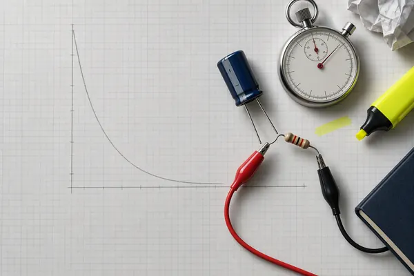
Synoptic links are common. The exponential form is the same as capacitor discharge, so make the comparison: λ plays the role of 1/CR, and the half-life corresponds to 0.693 CR. See capacitor discharge for the electrical version. Energy released in decay links to binding energy and mass defect, and radioactive tracers link to medical imaging such as PET. Logarithms and exponentials from your maths course appear here too, so be fluent with ln and e^x on your calculator.
Practice questions
A source has an activity of 3.6 × 10⁶ Bq and a decay constant of 4.0 × 10⁻⁴ s⁻¹. Calculate the number of undecayed nuclei and the half-life in minutes.3 marks
Show the answer
Answer: N = 9.0 × 10⁹; t½ = 29 minutes
N = A/λ = 3.6 × 10⁶ / 4.0 × 10⁻⁴ = 9.0 × 10⁹. t½ = ln 2 / λ = 0.693 / 4.0 × 10⁻⁴ = 1733 s = 28.9 min.
The corrected count rate from a source falls from 960 min⁻¹ to 120 min⁻¹ in 27 hours. Find the half-life.2 marks
Show the answer
Answer: 9.0 hours
960 to 120 is a factor of 8 = 2³, so three half-lives. t½ = 27 / 3 = 9.0 h.
What fraction of a radioactive sample remains after five half-lives? What fraction has decayed?2 marks
Show the answer
Answer: 1/32 = 0.031 remains; 31/32 = 0.97 has decayed
(½)⁵ = 1/32 = 0.03125. Decayed: 1 − 1/32 = 31/32 = 0.969.
A graph of ln (A / Bq) against t / h is a straight line through (0, 5.80) and (12, 3.40). Find the decay constant and the activity at t = 20 h.4 marks
Show the answer
Answer: λ = 0.20 h⁻¹; A = 6.0 Bq (to 2 s.f.)
Gradient = (3.40 − 5.80)/12 = −0.200, so λ = 0.200 h⁻¹. At t = 20 h, ln A = 5.80 − 0.200 × 20 = 1.80, so A = e^1.80 = 6.05 Bq, about 6.0 Bq.
An iterative model uses ΔN = −λNΔt with N₀ = 500, λ = 0.20 s⁻¹ and Δt = 0.50 s. Find N after three steps and compare with the exact value at t = 1.5 s.4 marks
Show the answer
Answer: Model: 364.5 (about 365). Exact: 370.
Each step multiplies N by 1 − 0.20 × 0.50 = 0.90. After 3 steps N = 500 × 0.9³ = 364.5. Exact: 500e^(−0.20 × 1.5) = 500e^(−0.30) = 370.4. The model is about 1.6% low.
Explain why measuring the background count rate over several minutes is better than over a few seconds.2 marks
Show the answer
Answer: Background is random, so a short count has a large percentage uncertainty; a long count averages out the fluctuations.
Counts follow a random pattern. More counts means a smaller fractional scatter, so the average rate is more reliable.
Next steps
Radioactive decay uses the same maths as capacitor discharge, so practise both together. Then look at where decay energy comes from in binding energy and mass defect, and at how radiation and sound are used in ultrasound and acoustic impedance for the medical imaging side. Browse everything in the Particles and medical physics module, or practise this topic with step-by-step marking.
Frequently asked questions
What is the difference between the decay constant and half-life?
The decay constant λ is the probability that a nucleus decays per second, so a large λ means fast decay. The half-life t½ is the time for half the nuclei to decay. They are linked by λt½ = ln 2, so a larger decay constant gives a shorter half-life.
Why is radioactive decay random?
There is no way to predict when a particular nucleus will decay. Each nucleus has the same chance per unit time, and the decay is not triggered by outside conditions. You can see this in the irregular clicks from a Geiger counter. Only large samples follow a smooth pattern.
How do you find half-life from a graph?
On a plot of activity against time, read the time for the activity to fall from any value to half of it and repeat from a second point to check. On a ln A against t graph, find the gradient, take its magnitude as λ, and use t½ = ln 2 / λ.
Why do we subtract background radiation?
Background radiation reaches the detector even when no source is present, so the raw count rate is too high. Subtracting the average background gives the count rate that comes from the source alone. Without this correction your half-life will come out too long.
How does carbon dating work?
Living organisms have a steady proportion of carbon-14. After death no more is taken in, so the activity per gram falls with a half-life of about 5730 years. The age follows from t = (1/λ) ln(A₀/A), using the activity of living material as A₀.
Do I need to remember the decay equations for OCR A?
Check your current data and formulae booklet to see which are given. Either way, you should be confident using A = λN, N = N₀e^(−λt) and λt½ = ln 2, and practise rearranging them with natural logs, because that is where marks are most often lost.
Related guides


Written for the OCR A Level Physics A (H556) specification. Questions are original and written in exam style; they are not taken from OCR papers. Spotted a mistake? Tell us.